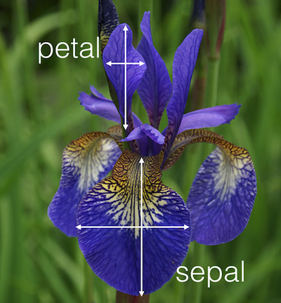
By combining multiple statistical techniques we created MLRP. In this post we will give a short overview of the technique by applying it to the iris data set (which can be found here), which is one of the best known data sets found in the classification and pattern recognition literature. The data consists of 150 observations of iris plants, which were measured in terms of sepal length (SL), sepal width (SW), petal length (PL), and petal width (PW).
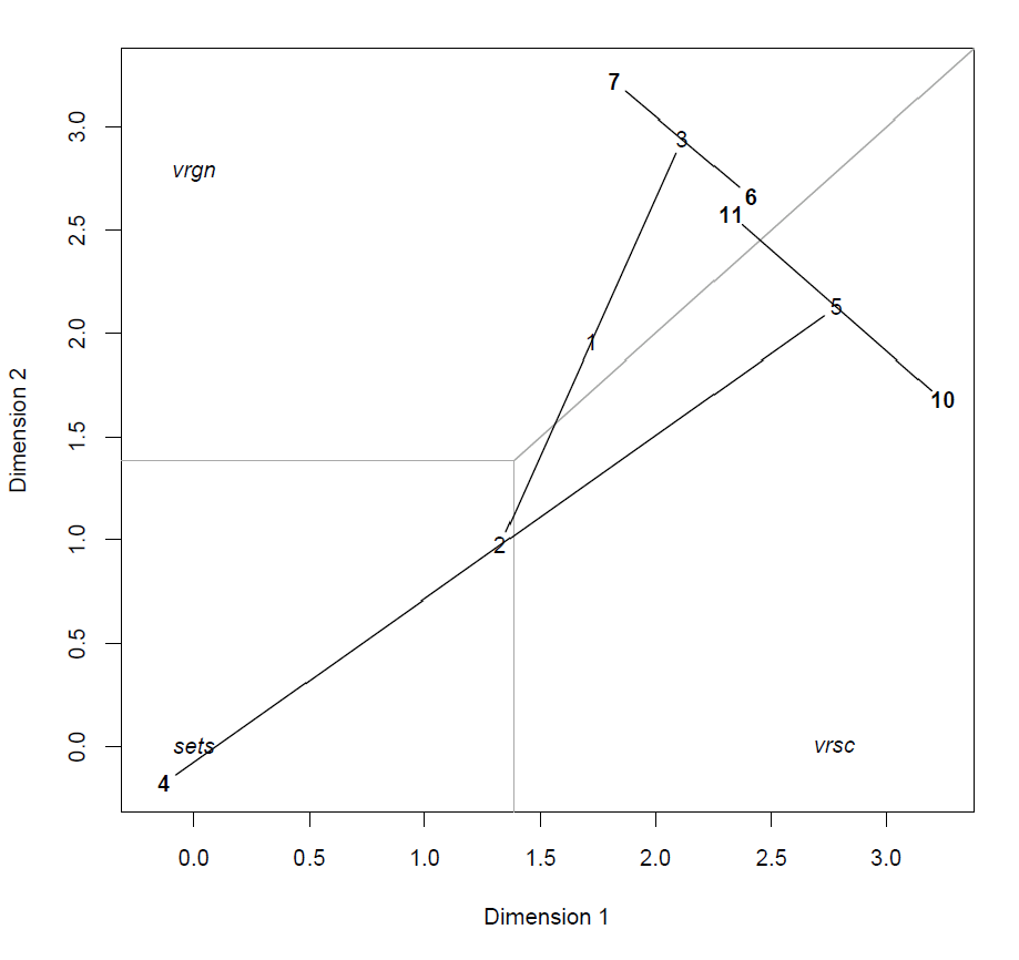
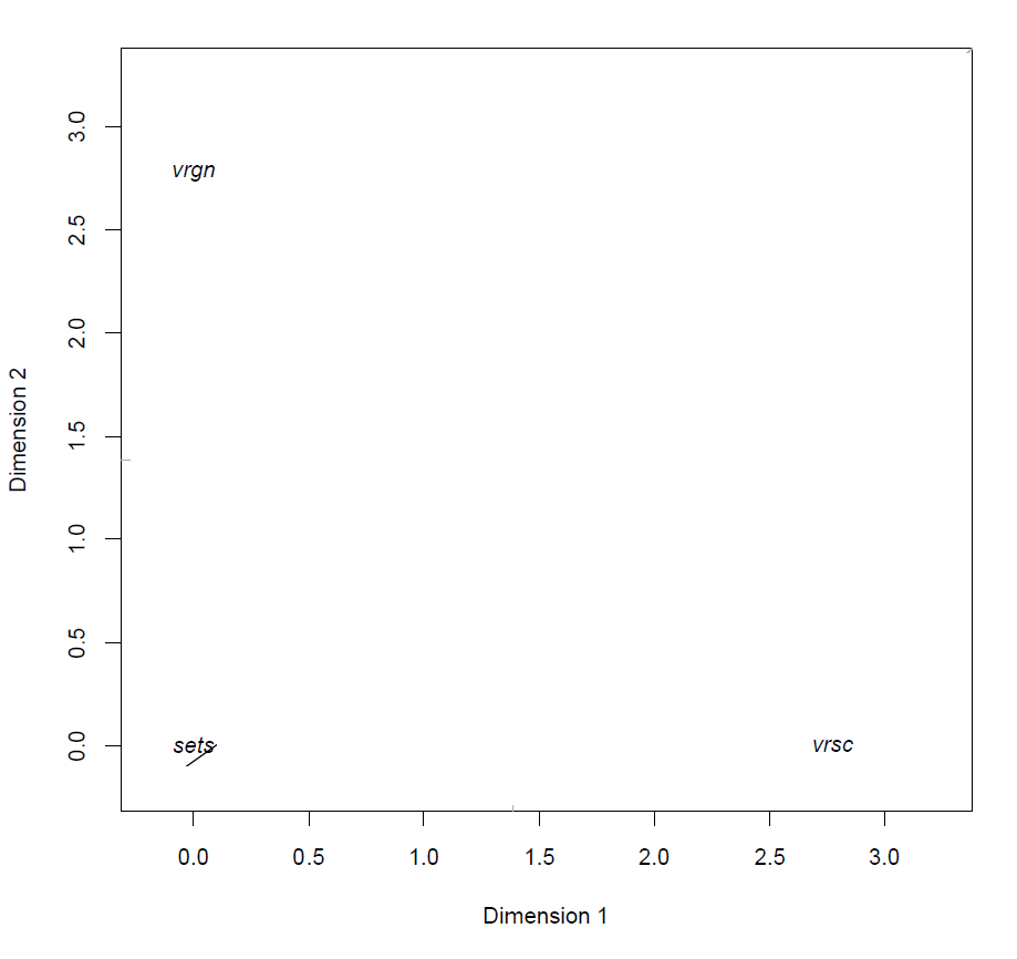
The outcome classes are species of iris plants: Setosa (sets), Versicolour (vrsc), and Virginica (vrgn).

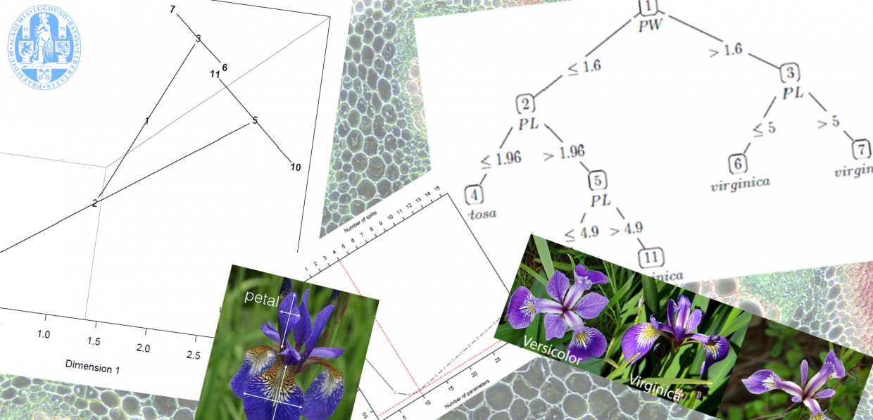
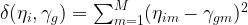
Below is a visual representation of the model fitted on a set of measurements of iris flowers.
MLRP model of Iris data
We will explain the technique by looking at the various components of the figure above and how these interact in the model.
Model components
The maximum dimensionality is dependent on the number of outcome classes (
Model space
There are 2 key component in the model which determine the class probability of an observation, namely the class point (

The subject points are the locations of the subjects (different Iris plants) within the model space. The coordinate for subject 


where 


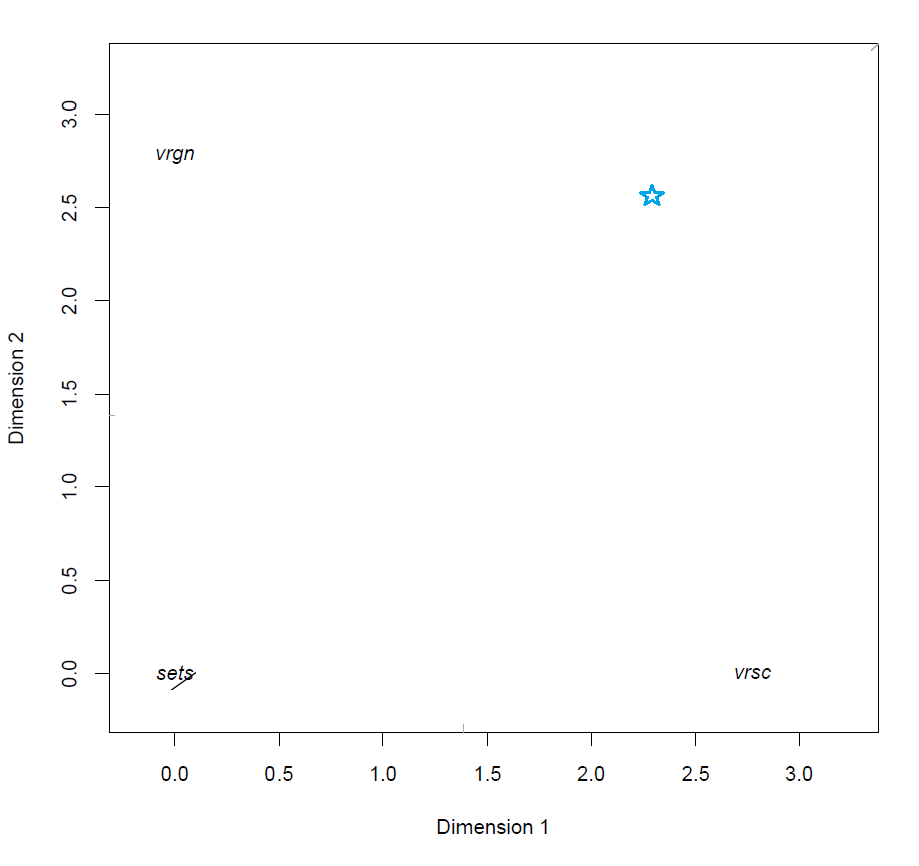
Subject point
The class probability is computed by the relative distance of the subject point and all the class points:
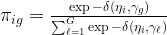

distance between the subject (

that:
Distance between subject and class points
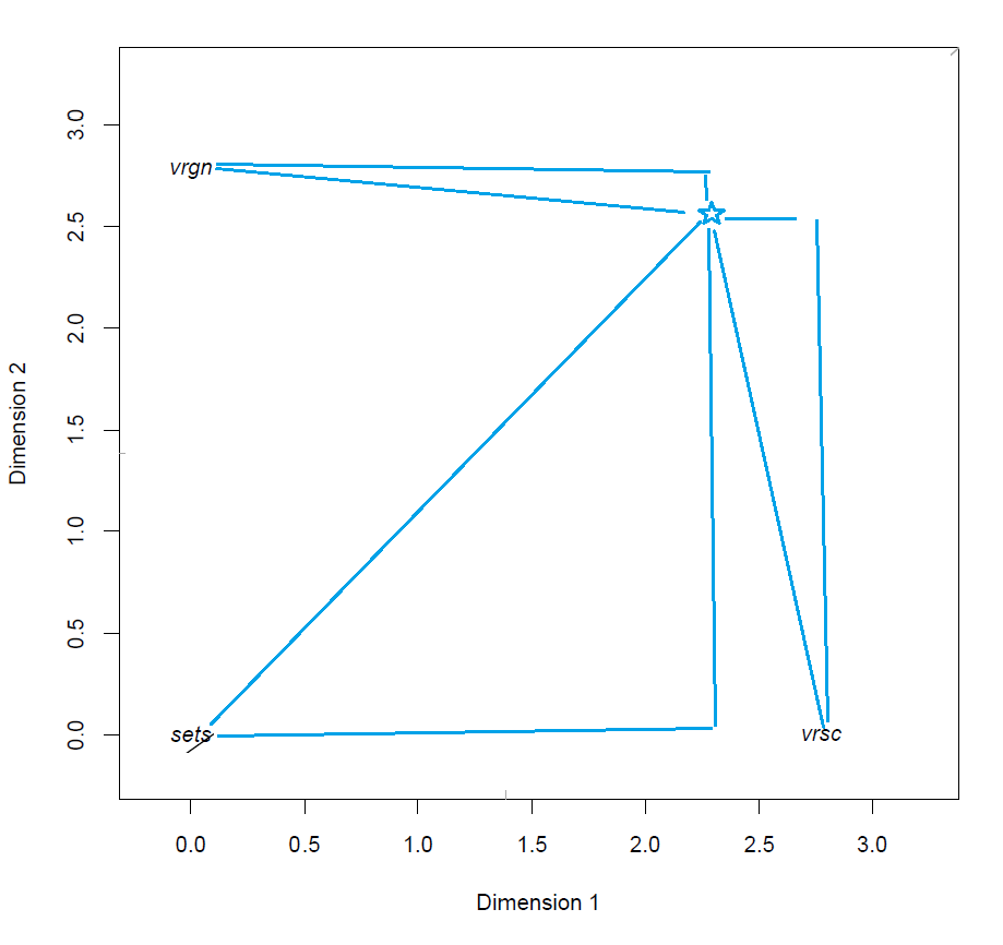
This means that the predicted class of a subject is the class corresponding to the closest class point of a subject. This is made clear in the model visualization by drawing the gray lines to represent the decision boundaries between the classes, such that subjects which fall within that region have the highest (predicted) probability of belonging to that class.
Class regions
Modeling procedure
As described before, the location of the subject is modelled. Originally the subject observations were used, but in this new technique we created sub-groups of observations and project these in the model space. This procedure of partitioning data in order to classify subjects is also used in the construction of decision trees, in which the data is recursively partitioned in sub-groups in order to obtain more homogeneous sets of subjects with respect to the outcome classes.
In this approach, the tree is built such that the split is selected which maximizes the log-likelihood. After a new split is found, and thus new branches are formed, the location of the new nodes is optimized by (re)estimating the regression weights
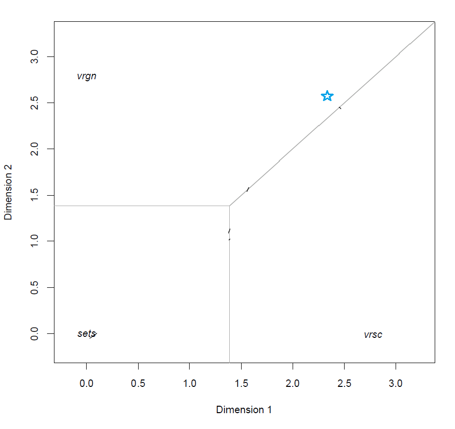
AIC values during model development
In the graph above it can be seen that the AIC value quickly improves in the first few steps. After the optimal value at 4 splits, the performance measure steadily deteriorates as more splits are added to the model. The resulting tree model is represented below.
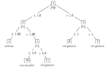
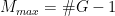
Iris tree model
In order to classify a subject we start at the top: if the petal width 
The class membership is estimated based on the distance framework discussed above and the tree can therefore be represented in the model space with the following figure.
MLRP model of Iris data
In this visualization we see that the trunk of the tree is located in the Virginica region. When the first split is evaluated and the pedal width